Wurm lab: home | |

Reads to reference genome & gene predictions

Introduction

Cheap sequencing has created the opportunity to perform molecular-genetic analyses on just about anything. Conceptually, doing this would be similar to working with traditional genetic model organisms. But a large difference exists: For traditional genetic model organisms, large teams and communities of expert assemblers, predictors, and curators have put years of efforts into the prerequisites for most genomic analyses, including a reference genome and a set of gene predictions. In contrast, those of us working on “emerging” model organisms often have limited or no pre-existing resources and are part of much smaller teams.

The steps below are meant to provide some ideas that can help obtain a reference genome and a reference geneset of sufficient quality for ecological and evolutionary analyses. They are based on (but updated from) work we did for the fire ant genome.

Specifically, focusing on low coverage of ~0.5% of the fire ant genome, we will:

inspect and clean short (Illumina) reads,
perform genome assembly,
assess the quality of the genome assembly using simple statistics,
predict protein-coding genes,
assess quality of gene predictions,
assess quality of the entire process using a biologically meaning measure.

Please note that these are toy/sandbox examples simplified to run on laptops and to fit into the short format of this course. For real projects, much more sophisticated approaches are needed!

Set up directory hierarchy to work in

All work must be done in home directory. First, copy over the input files from HPC to your local PC:

rmdir hpc # remove previous directory
scp -r login2.hpc.qmul.ac.uk:/data/SBCS-MSc-BioInf/data ~/2017-09-BIO721_genome_bioinformatics_input
chmod a-w -R ~/2017-09-BIO721_genome_bioinformatics_input

Check that you have a directory called ~/2017-09-BIO721_genome_bioinformatics_input. If not, ask for help.

Start by creating a directory to work in. Drawing on ideas from Noble (2009) and others, we recommend following a specific convention for all your projects.

For this, create a main directory for this section of the course (~/2017-09-29-reference_genome), and create relevant input and results subdirectories.

For each step that we will perform, you should:

have input data in a relevant subdirectory
work in a relevant subdirectory

And each directory in which you have done something should include a WHATIDID.txt file in which you log your commands.

Being disciplined about this is extremely important. It is similar to having a laboratory notebook. It will prevent you from becoming overwhelmed by having too many files, or not remembering what you did where.

Sequencing an appropriate sample

Less diversity and complexity in a sample makes life easier: assembly algorithms really struggle when given similar sequences. So less heterozygosity and fewer repeats are easier. Thus:

A haploid is easier than a diploid (those of us working on haplo-diploid Hymenoptera have it easy because male ants are haploid).
It goes without saying that a diploid is easier than a tetraploid!
An inbred line or strain is easier than a wild-type.
A more compact genome (with less repetitive DNA) is easier than one full of repeats - sorry, grasshopper & Fritillaria researchers!

Many considerations go into the appropriate experimental design and sequencing strategy. We will not formally cover those here & instead jump right into our data.

Part 1: Short read cleaning

Sequencers aren’t perfect. All kinds of things can and do go wrong. “Crap in – crap out” means it’s probably worth spending some time cleaning the raw data before performing real analysis.

Short read cleaning

Sequencers aren’t perfect. All kinds of things can and do go wrong. “Crap in – crap out” means it’s probably worth spending some time cleaning the raw data before performing real analysis.

Initial inspection

FastQC (documentation) can help you understand sequence quality and composition, and thus can inform read cleaning strategy.

Link the raw sequence files (~/2017-09-BIO721_genome_bioinformatics_input/reads.pe*.fastq.gz) to a relevant input directory (e.g., ~/2017-09-29-reference_genome/input/01-read_cleaning/).

Now move to a relevant results directory (e.g., ~/2017-09-29-reference_genome/results/01-read_cleaning/).

Here, run FastQC on the reads.pe2 file. The --outdir option will help you clearly separate input and output files (and remember to log the commands you used in the WHATIDID.txt file).

Your resulting directory structure, should look like this:

tree -h
.
├── [4.0K]  input
│   └── [4.0K]  01-read_cleaning
│       ├── [  53]  reads.pe1.fastq.gz
│       ├── [  53]  reads.pe2.fastq.gz
│       └── [  44]  WHATIDID.txt
└── [4.0K]  results
    └── [4.0K]  01-read_cleaning
        ├── [  28]  input -> ../../input/01-read_cleaning/
        ├── [336K]  reads.pe2_fastqc.html
        ├── [405K]  reads.pe2_fastqc.zip
        └── [ 126]  WHATIDID.txt

What does the FastQC report tell you? (the documentation clarifies what each plot means). For comparison, have a look at some plots from other sequencing libraries: e.g, [1], [2], [3].

Decide whether and how much to trim from the beginning and end of our sequences. What else might you want to do?

Below, we will perform three cleaning steps:

Trimming the ends of sequence reads using seqtk.
K-mer filtering using khmer.
Removing sequences that are of low quality or too short using seqtk.

Other tools including fastx_toolkit, kmc2 and Trimmomatic can also be useful.

Trimming

seqtk (documentation) is a fast and lightweight tool for processing FASTA and FASTQ sequences.

Based on the results from FastQC, replace REPLACE and REPLACE below to appropriately trim from the beginning (-b) and end (-e) of the sequences.

seqtk trimfq -b REPLACE -e REPLACE input/reads.pe2.fastq.gz > tmp/reads.pe2.trimmed.fq

This will only take a few seconds (make sure you replaced REPLACE).

Let’s similarly inspect the paired set of reads, reads.pe1, and appropriately trim them.

seqtk trimfq -b REPLACE -e REPLACE input/reads.pe1.fastq.gz > tmp/reads.pe1.trimmed.fq

K-mer filtering, removal of low quality and short sequences

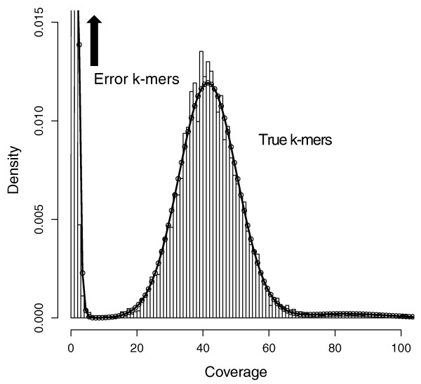
Say you have sequenced your sample at 45x genome coverage. The real coverage distribution will be influenced by factors including DNA quality, library preparation type and local GC content, but you might expect most of the genome to be covered between 20 and 70x. In practice, the distribution can be very strange. One way of rapidly examining the coverage distribution before you have a reference genome is to chop your raw sequence reads into short “k-mers” of 31 nucleotides, and count how often you get each possible k-mer. Surprisingly,

many sequences are extremely rare (e.g., present only once). These are likely to be errors that appeared during library preparation or sequencing, or could be rare somatic mutations). Such sequences can confuse assembly software; eliminating them can decrease subsequent memory & CPU requirements.
Other sequences may exist at 10,000x coverage. These could be pathogens or repetitive elements. Often, there is no benefit to retaining all copies of such sequences because the assembly software will be confused by them; while retaining a small proportion could of such reads could significantly reduce CPU, memory and space requirements.

An example plot of a k-mer frequencies from a haploid sample sequenced at ~45x coverage:

kmer distribution graph from UCSC

It is possible to count and filter “k-mers” using khmer (documentation; the kmc2 tool is faster and thus can be more appropriate for large datasets).

Below, we use khmer to remove extremely frequent k-mers (more than 100x), remove extremely rare k-mers, and we use seqtk to truncate sequences containing unresolved “N”s and nucleotides of particularly low quality. After all this truncation and removal, seqtk remove reads that have become too short, or no longer have a paired read. Understanding the exact commands – which are a bit convoluted – is unnecessary. It is important to understand the concept of k-mer filtering.

# 1. Interleave Fastqs (khmer needs both paired end files merged into one file)
seqtk mergepe tmp/reads.pe1.trimmed.fq tmp/reads.pe2.trimmed.fq > tmp/reads.pe12.trimmed.fq

# 2. Remove coverage above 100x, save kmer.counts table
khmer normalize-by-median.py -p --ksize 20 -C 100 -M 1e9 -s tmp/kmer.counts \
                -o tmp/reads.pe12.trimmed.max100.fq tmp/reads.pe12.trimmed.fq
# 3. Filter low abundance kmers
khmer filter-abund.py -V tmp/kmer.counts \
                      -o tmp/reads.pe12.trimmed.max100.norare.fq \
                      tmp/reads.pe12.trimmed.max100.fq
# 4. Remove low quality bases, short sequences, and non-paired reads
seqtk seq -q 10 -N -L 80 tmp/reads.pe12.trimmed.max100.norare.fq | \
                 seqtk dropse > tmp/reads.pe12.trimmed.max100.norare.noshort.fq

# 5. De-interleave filtered reads
khmer split-paired-reads.py tmp/reads.pe12.trimmed.max100.norare.noshort.fq -d tmp/

# 6. Rename output reads to something more human-friendly
ln -s tmp/reads.pe12.trimmed.max100.norare.noshort.fq.1 reads.pe1.clean.fq
ln -s tmp/reads.pe12.trimmed.max100.norare.noshort.fq.2 reads.pe2.clean.fq

Inspecting quality of cleaned reads

Which percentage of reads have we removed overall? (hint: wc -l can count lines in a non-gzipped file). Is there a general rule about how much we should be removing? Run fastqc again, this time on reads.pe2.clean.fq. Which statistics have changed? Does the “per tile” sequence quality indicate to you that we should perhaps do more cleaning?