Reads to reference genome & gene predictions
Introduction
Cheap sequencing has created the opportunity to perform molecular-genetic analyses on just about anything. Conceptually, doing this would be similar to working with traditional genetic model organisms. But a large difference exists: For traditional genetic model organisms, large teams and communities of expert assemblers, predictors, and curators have put years of efforts into the prerequisites for most genomic analyses, including a reference genome and a set of gene predictions. In contrast, those of us working on “emerging” model organisms often have limited or no pre-existing resources and are part of much smaller teams.
The steps below are meant to provide some ideas that can help obtain a reference genome and a reference geneset of sufficient quality for ecological and evolutionary analyses. They are based on (but updated from) work we did for the fire ant genome.
Specifically, focusing on low coverage of ~0.5% of the fire ant genome, we will:
- inspect and clean short (Illumina) reads,
- perform genome assembly,
- assess the quality of the genome assembly using simple statistics,
- predict protein-coding genes,
- assess quality of gene predictions,
- assess quality of the entire process using a biologically meaning measure.
Please note that these are toy/sandbox examples simplified to run on laptops and to fit into the short format of this course. For real projects, much more sophisticated approaches are needed!
Preparation
Once you’re logged into the virtual machine, create a directory to work in. Drawing on ideas from Noble (2009) and others, we recommend following a specific convention for all your projects. For example, create a main directory for this section of the course (e.g., ~/2016-05-30-reference), and create relevant subdirectories for each step (e.g., first one might be ~/2016-05-30-reference/results/01-read_cleaning).
We similarly recommend that you log your commands in a WHATIDID.txt file in each directory.
Sequencing an appropriate sample
Less diversity and complexity in a sample makes life easier: assembly algorithms really struggle when given similar sequences. So less heterozygosity and fewer repeats are easier. Thus:
- A haploid is easier than a diploid (those of us working on haplo-diploid Hymenoptera have it easy because male ants are haploid).
- It goes without saying that a diploid is easier than a tetraploid!
- An inbred line or strain is easier than a wild-type.
- A more compact genome (with less repetitive DNA) is easier than one full of repeats - sorry, grasshopper & Fritillaria researchers!
Many considerations go into the appropriate experimental design and sequencing strategy. We will not formally cover those here & instead jump right into our data.
Short read cleaning
Sequencers aren’t perfect. All kinds of things can and do go wrong. “Crap in – crap out” means it’s probably worth spending some time cleaning the raw data before performing real analysis.
Initial inspection
FastQC (documentation) can help you understand sequence quality and composition, and thus can inform read cleaning strategy.
Move, copy or link the raw sequence files (~/data/reference_assembly/reads.pe*.fastq.gz) to a relevant input directory (e.g. ~/2016-05-30-reference/data/01-read_cleaning/). Now run FastQC on the reads.pe2 file. The --outdir option will help you clearly separate input and output files.
If respecting our project structure convention, your resulting directory structure may look like this:
user@userVM:~/2016-05-30-assembly$ tree -h
.
├── [4.0K]  data
│   └── [4.0K]  01-read_cleaning
│       ├── [  53]  reads.pe1.fastq.gz -> /home/user/data/reference_assembly/reads.pe1.fastq.gz
│       ├── [  53]  reads.pe2.fastq.gz -> /home/user/data/reference_assembly/reads.pe2.fastq.gz
│       └── [  44]  WHATIDID.txt
└── [4.0K]  results
    └── [4.0K]  01-read_cleaning
        ├── [  28]  input -> ../../data/01-read_cleaning/
        ├── [336K]  reads.pe2_fastqc.html
        ├── [405K]  reads.pe2_fastqc.zip
        └── [ 126]  WHATIDID.txt
What does the FastQC report tell you? (the documentation clarifies what each plot means). For comparison, have a look at some plots from other sequencing libraries: e.g, [1], [2], [3].
![[1]](/genomicscourse/2016-SIB/practicals/reference_genome/img-qc/per_base_quality.png)
![[2]](/genomicscourse/2016-SIB/practicals/reference_genome/img-qc/qc_factq_tile_sequence_quality.png)
![[3]](/genomicscourse/2016-SIB/practicals/reference_genome/img-qc/per_base_sequence_content.png)
Decide whether and how much to trim from the beginning and end of our sequences. What else might you want to do?
Below, we will perform three cleaning steps:
- Trimming the ends of sequence reads using seqtk.
- K-mer filtering using khmer.
- Removing sequences that are of low quality or too short using seqtk.
Other tools including fastx_toolkit, kmc2 and Trimmomatic can also be useful.
Trimming
seqtk (documentation) is a fast and lightweight tool for processing FASTA and FASTQ sequences.
Based on the results from FastQC, replace REPLACE and REPLACE below to appropriately trim from the beginning (-b) and end (-e) of the sequences.
seqtk trimfq -b REPLACE -e REPLACE input/reads.pe2.fastq.gz | gzip > tmp/reads.pe2.trimmed.fq.gz
This will only take a few seconds (make sure you replaced REPLACE).
Let’s similarly filter the paired set of reads, reads.pe1:
seqtk trimfq -b 5 -e 5 input/reads.pe1.fastq.gz | gzip > tmp/reads.pe1.trimmed.fq.gz
K-mer filtering, removal of low quality and short sequences
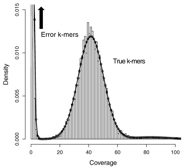
Say you have sequenced your sample at 45x genome coverage. The real coverage distribution will be influenced by factors including DNA quality, library preparation type and local GC content, but you might expect most of the genome to be covered between 20 and 70x. In practice, the distribution can be very strange. One way of rapidly examining the coverage distribution before you have a reference genome is to chop your raw sequence reads into short “k-mers” of 31 nucleotides, and count how often you get each possible k-mer. Surprisingly,
- many sequences are extremely rare (e.g., once). These are likely to be errors that appeared during library preparation or sequencing, or could be rare somatic mutations). Such sequences can confuse assembly software; eliminating them can decrease subsequent memory & CPU requirements.
- Other sequences may exist at 10,000x coverage. These could be pathogens or repetitive elements. Often, there is no benefit to retaining all copies of such sequences because the assembly software will be confused by them; while retaining a small proportion could of such reads could significantly reduce CPU, memory and space requirements.
An example plot of a k-mer frequencies from a haploid sample sequenced at ~45x coverage:
It is possible to count and filter “k-mers” using khmer (documentation; the kmc2 tool is faster and thus can be more appropriate for large datasets.
Below, we use khmer to remove extremely frequent k-mers (more than 100x), remove extremely rare k-mers, and we use seqtk to truncate sequences containing unresolved “N”s and nucleotides of particularly low quality. After all this truncation and removal, seqtk remove reads that have become too short, or no longer have a paired read. Understanding the exact commands – which are a bit convoluted – is unnecessary. It is important to understand the concept of k-mer filtering.
# 1. Interleave Fastqs (khmer needs both paired end files merged into one file
seqtk mergepe tmp/reads.pe1.trimmed.fq.gz tmp/reads.pe2.trimmed.fq.gz > tmp/reads.pe12.trimmed.fq

# 2. Remove coverage above 100x, save kmer.counts table
khmer normalize-by-median.py -p --ksize 20 -C 100 -M 1e9 -s tmp/kmer.counts \
                -o tmp/reads.pe12.trimmed.max100.fq tmp/reads.pe12.trimmed.fq
# 3. Filter low abundance kmers
khmer filter-abund.py -V tmp/kmer.counts \
                      -o tmp/reads.pe12.trimmed.max100.norare.fq \
                      tmp/reads.pe12.trimmed.max100.fq
# 4. Remove low quality bases, short sequences, and non-paired reads
seqtk seq -q 10 -N -L 80 tmp/reads.pe12.trimmed.max100.norare.fq | \
                 seqtk dropse > tmp/reads.pe12.trimmed.max100.norare.noshort.fq

# 5. De-interleave filtered reads
khmer split-paired-reads.py tmp/reads.pe12.trimmed.max100.norare.noshort.fq -d tmp/

# 6. Rename output reads to something more human-friendly
ln -s tmp/reads.pe12.trimmed.max100.norare.noshort.fq.1 reads.pe1.clean.fq
ln -s tmp/reads.pe12.trimmed.max100.norare.noshort.fq.2 reads.pe2.clean.fq
Inspecting quality of cleaned reads
Which percentage of reads have we removed overall? (hint: wc -l can count lines in a non-gzipped file). Is there a general rule about how much we should be removing?
Run fastqc again, this time on reads.pe2.clean.fq. Which statistics have changed? Does the “per tile” sequence quality indicate to you that we should perhaps do more cleaning?
Genome assembly
Offline exercise
Find (or make) four friends; find a table. In groups of 4 or 5, ask an assistant for an assembly task.
Brief assembly example / concepts
Many different pieces of software exist for genome assembly.
If we wanted to assemble our cleaned reads with SOAPdenovo, we would (in a new results/02-assembly directory) create a soap_config.txt file containing the following:
max_rd_len=101          # maximal read length
[LIB]            # One [LIB] section per library
avg_ins=470             # average insert size
reverse_seq=0           # if sequence needs to be reversed
asm_flags=3             # use for contig building and subsequent scaffolding
rank=1                  # in which order the reads are used while scaffolding
q1=input/reads.pe1.clean.fq
q2=input/reads.pe2.clean.fq
Then run the following line. THIS IS RAM-INTENSE – with only 2Gb ram, your computer may struggle - you don’t need to do this and can just download the result!
soapdenovo2-63mer all -s soap_config.txt -K 63 -R -o assembly
Like any other assembler, SOAPdenovo creates many files, including an assembly.scafSeq file that is likely to be used for follow-up analyses. You can download it here. Why does this file contain so many NNNN sequences?
There are many other genome assembly approaches. While waiting for everyone to make it to this stage, try to understand some of the challenges of de novo genome assembly and the approaches used to overcome them via the following papers:
- Genetic variation and the de novo assembly of human genomes. Chaisson et al 2015 NRG (to overcome the paywall, login via your university, email the authors, or try scihub.
- The now slightly outdated (2013) Assemblathon paper.
- Metassembler: merging and optimizing de novo genome assemblies. Wences & Schatz (2015).
- A hybrid approach for de novo human genome sequence assembly and phasing. Mostovoy et al (2016).
Quality assessment
How do we know if our genome is good?
“… the performance of different *de novo genome assembly algorithms can vary greatly on the same dataset, although it has been repeatedly demonstrated that no single assembler is optimal in every possible quality metric [6, 7, 8]. The most widely used metrics for evaluating an assembly include 1) contiguity statistics such as scaffold and contig N50 size, 2) accuracy statistics such as the number of structural errors found when compared with an available reference genome (GAGE (Genome Assembly Gold Standard Evaluation) evaluation tool [8]), 3) presence of core eukaryotic genes (CEGMA (Core Eukaryotic Genes Mapping Approach) [9]) or, if available, transcript mapping rates, and 4) the concordance of the sequence with remapped paired-end and mate-pair reads (REAPR (Recognizing Errors in Assemblies using Paired Reads) [10], assembly validation [11], or assembly likelihood [12]).”* - Wences & Schatz (2015)
Simple metrics
An assembly software will generally provide some statistics about what it did. But the output formats differ between assemblers. Quast, the Quality Assessment Tool for Genome Assemblies creates a standardized report. Run Quast (available at ~/software/quast-4.0/quast.py) on the assembly.scafSeq file. No special options - just the simple scenario to get some statistics.
Have a look at the report (pdf or html) Quast generated.
What do the values in the table mean? For which ones is higher better, and for which ones is smaller better? Is Quast’s use of the word “contig” appropriate?
Perhaps we have prior knowledge about the %GC content to expect, the number of chromosomes to expect, and the total genome size – these can inform comparisons with output statistics present in Quast’s report.
Biologically meaningful measures
Unfortunately, with many of the simple metrics, it is difficult to determine whether the assembler did things correctly, or just haphazardly stuck lots of reads together!
We probably have other prior information about what to expect in this genome. For example:
- If we have a reference assembly from a no-too-distant relative, we could expect large parts of genome to be organised in the same order, i.e., synteny.
- If we independently created a transcriptome assembly, we can expect the exons making up each transcript to map sequentially onto the genome (see TGNet for an implementation).
- We can expect the different scaffolds in the genome to have a unimodal distribution in sequence read coverage. Similarly, one can expect GC% to be unimodally distributed among scaffolds. Using this idea, the Blobology approach determined that evidence of foreign sequences in Tardigrades is largely due to extensive contamination rather than extensive horizontal gene transfer Koutsovoulos et al 2016.
- We can expect different patterns of gene content and structure between eukaryotes and prokaryotes.
- Pushing this idea further, we can expect a genome to contain a single copy of each of the “house-keeping” genes found in related species. We will see how to apply this idea using BUSCO (Benchmarking Universal Single-Copy Orthologs) later today (after we know how to obtain gene predictions). Note that:
- BUSCO is a refined, modernized implementation of the CEGMA (Core Eukaryotic Genes Mapping Approach). CEGMA examines a eukaryotic genome assembly for presence and completeness of 248 “core eukaryotic genes”.
- QUAST also includes a “quick and dirty” method of finding genes.
Gene prediction
Many tools exist for gene prediction, some based on ab initio statistical models of what a protein-coding gene should look like, others that use similarity with protein-coding genes from other species, and others (such as Augustus and SNAP), that use both. There is no perfect tool or approach, thus we typically run many gene-finding tools and call a consensus between the different predicted gene models. MAKER and JAMg can do this for us. Let’s use MAKER on a sandbox example.
Start in a new directory (e.g., ~/2016-05-30-reference/results/03-gene_prediction). Pull out the longest few scaffolds from the assembly.scafSeq (e.g., using seqtk seq -L 20000) into their own fasta (e.g., min20000.fa).
Running maker -OPTS will generate an empty maker_opts.ctl configuration file (ignore the warning). Edit that file to specify:
- genome:
min20000.fa - augustus species:
honeybee1(yes that’s a 1; check~/software/augustus-3.2.1/config/species/for a full list of Augustus’ built-in HMM gene models) - deactivate RepeatMasker by replacing
model_org=alltomodel_org=(i.e., nothing)
For a real project, we would use include RepeatMasker (perhaps after creating a new repeat library), would provide as much relevant information as possible (e.g., RNAseq read mappings, transcriptome assembly – both improve gene prediction performance tremendously), and iteratively train gene prediction algorithms for our data including Augustus and SNAP.
Run maker maker_opts.ctl. This may take a few minutes, depending on how much data you gave it.
Once its done the results will be hidden in subdirectories of *maker.output/min20k_datastore. Perhaps its easier to find the gene predictions using find then grep for gff or proteins. You can ignore the (temporary) contents under theVoid directories.
Quality control of individual genes
So now we have some gene predictions… how can we know if they are any good? The easiest way to get a feel for this is by comparing a few of them (backup examples)) to known sequences from other species. For this, launch a local BLAST server to compare a few of your protein-coding gene predictions to the high quality predictions in swissprot:
sequenceserver -d ~/data/reference_databases
Do any of these genes have significant similarity to known sequences? For a give gene prediction, do you think it is complete, or can you infer from the BLAST alignments that something may be wrong?
As you can see, gene prediction software is imperfect – this is even the case when using all available evidence. This is potentially costly for analyses that rely on gene predictions - i.e. many of the anlyses we might want to do!
“Incorrect annotations [ie. gene identifications] poison every experiment that makes use of them. Worse still the poison spreads.” – Yandell & Ence (2012).
The GeneValidator tool can help to evaluate quality of a gene prediction by comparing features of a gene prediction to similar database sequences. This approach expects that similar sequences should for example be of similar length.
You can simply run genevalidator -d ~/data/reference_databases/uniprot/uniprot_sprot.fasta proteins.fasta (on your gene predictions, or these examples), or use the web service for queries of few sequences. Alternatively just check the screenshots linked in the next sentence. Try to understand why some gene predictions have no reason for concern (e.g.), while others do (e.g.).
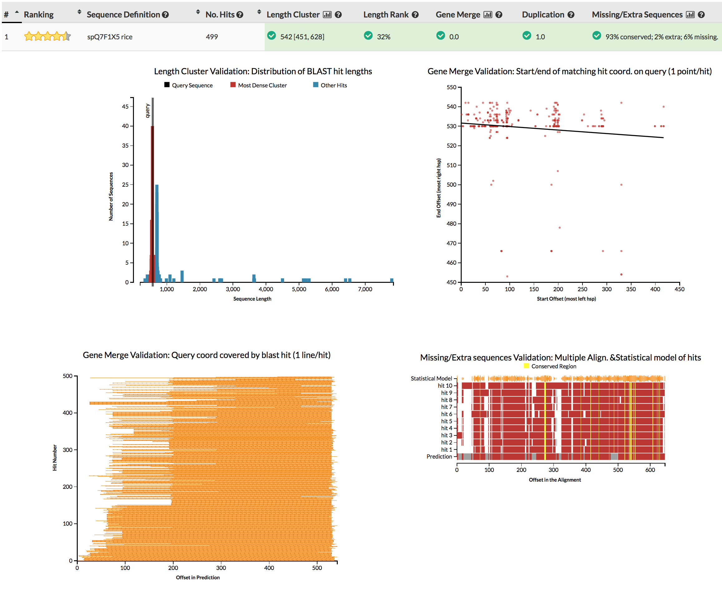
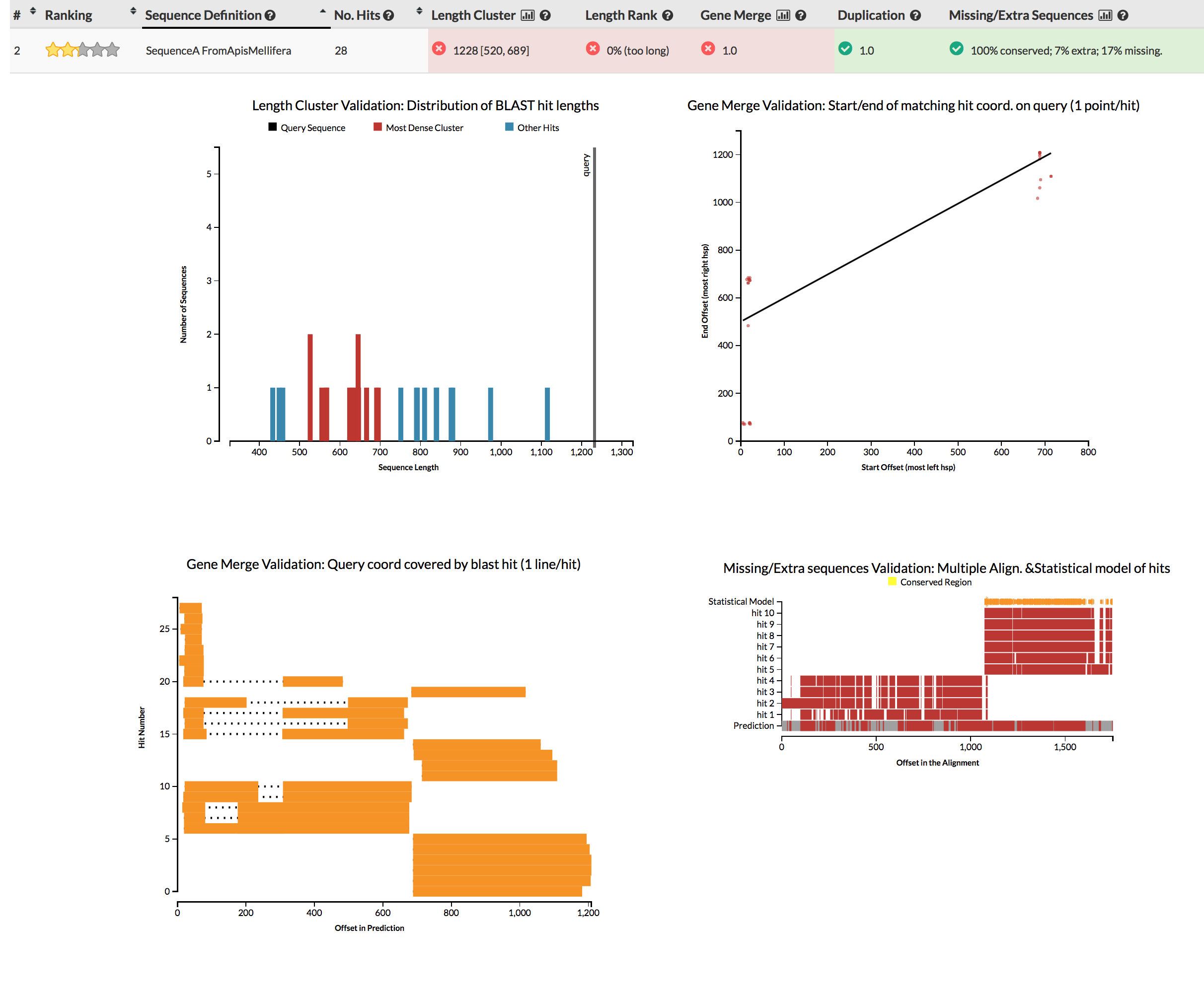
Comparing whole genesets & prioritizing genes for manual curation
Genevalidator’s visual output can be handy when looking at few genes. But the tool also provides tab-delimited output, handy when working in the command-line or when running the software on whole proteomes. For example, this can help analysis:
- in situations when you can choose between mulitple gene sets.
- or to identify which gene predictions are likely ok, and which need to be inspected and potentially manual fixed.
Manual curation
Because automated gene predictions aren’t perfect, manual inspection and fixing are often required. The most commonly used software for this is Apollo/WebApollo. We have no time for manual curation today, so here’s simply a screenshot:
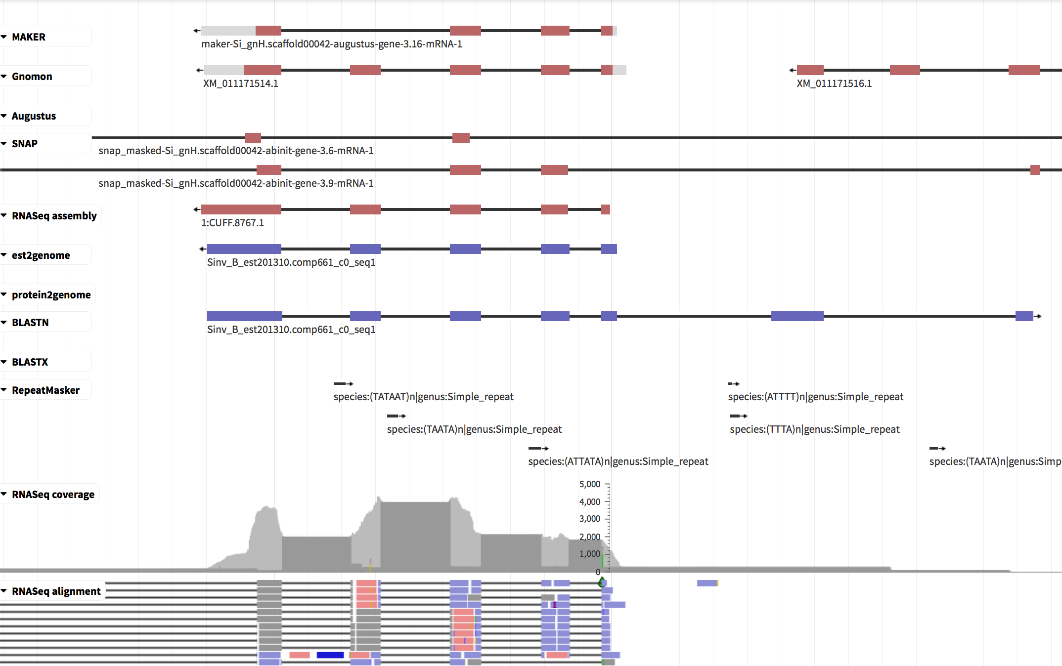
The interface shows the genome sequence horizontally (nucleotides only visible when zooming in), similarly to a genome browser.
- the top line shows the MAKER consensus gene model which includes 4 exons.
- some of the evidence tracks show 5 exons; while e.g. SNAP shows two models (with 2 and 3 exons on-screen) and suggests that the gene has additional exons beyond the limits of the screenshot.
- RNAseq reads provide extensive support that the gene has 5 exons, not 4.
Using curation software, you can edit the gene prediction: add or remove exons, merge or split gene models, and adjust exon boundaries.
Quality control of the whole process
Congrats on getting from sequence reads to a genome assembly and gene predictions! We can now move on to quality-controlling our whole process by testing for the presence of single-copy-orthologs with BUSCO.